How to make a chart on Google Sheets

How to make a chart on Google Sheets – For your personal project, you need to collect some data and represent them in a graphic. To do this, you were advised to use Google Sheets, a free tool offered by Google that, in fact, allows you to create and customize online spreadsheets. Without having to repeat it twice, you created a new document and entered all your data without encountering any kind of problem: unfortunately, however, you did not have the same luck when you tried to add a new chart.

Contents hide

1 Index

2 How to make a chart on Google Sheets from PC

3 How to make a chart on Google Sheets from the app

3.1 Related posts:

That’s the way it is, right? Then let me tell you that you’ve come to the right place at the right time! In the next paragraphs of this tutorial, in fact, I will explain to you how to make a chart on Google Sheets providing you with all the information you need to succeed in your intent. In addition to the detailed procedure for creating a new graph with the data of your interest, both from a computer and from a smartphone and tablet, you will also find all the instructions to customize it as you prefer.

If you are ready to deepen the subject, all you have to do is take five minutes of free time and dedicate yourself to reading the next paragraphs. I assure you that, by carefully following the instructions I am about to give you and trying to put them into practice from the device of your interest, creating and personalizing a chart on Google Sheets will be really a breeze. Let it bet?

Index

How to make a chart on Google Sheets from PC

The procedure for make a chart on Google Sheets it’s pretty simple. All you need to do is select the cells containing the data you want to include in the chart and hit the option to create one. Later, you can manage its style and colors, enter a title to display in the chart and apply further changes.

To proceed from computer, linked to the main page of Google Sheets and, if you have not already done so, log in with your Google account by pressing the button Log in, selecting theaccount Google of your interest from the box that opens and inserting the password in the appropriate field. If, on the other hand, you have not yet associated a Google account with your browser, select the option Add another account, enter the relevant email address in the field Email address or telephone number, type the password in the field Enter your password and click on the button Forward, to login.

Read This Now: Boot your Mac from a USB drive - Easy Steps

At this point, click on the option Empty, if you want to create a blank spreadsheet. Alternatively, select one of the ready-to-use spreadsheet templates (ex. Monthly budget, Annual budget, Weekly schedule, Expense statement etc.) or, if you have already created a file before and now want to edit it, locate it in the section Precedents and click his Name, to open it.

Now, select all cells containing the data that you want to show in the graph (including those in which you have entered some text that you also want to display in the graph). For example, if you have created a worksheet to manage your annual budget and you want to display everything in a graph, select both the cells in which you have entered the data relating to enter, exits e earnings both the cells in which you entered the names of individual months.

If, on the other hand, continuing with the same example, you want to create a chart in which to display only the earnings per month, you must select only the cells relating to the names of the individual months and those relating to earnings.

In any case, after choosing the data to include in the graph, click on the item insert located at the top and select the option Graphic from the menu that opens. Alternatively, click on the item Insert chart (the icon of graphic) located in the Google Sheets toolbar.

Automatically, a column chart will be created with all the data you previously selected. Dragging one of the four squares placed in the corners of the graph inwards or outwards, you can decrease or increase the size of the graph itself, maintaining its proportions. Furthermore, by keeping the mouse clicked anywhere on the graph, you can move it to the position you prefer.

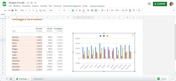
At this point, acting in the section Graphic editor pop-up on the right (if you do not see it, select the graph, press the icon of three dots and choose the option Edit chart from the menu that opens), you can configure and customize your chart.

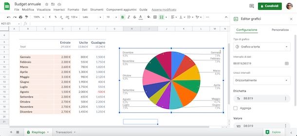
First, make sure the item is selected Configuration and, via the drop-down menu Type of chart, choose one of the available options (Line, Area, Column, bar, Map, Dispersion etc.) to choose the type of chart you prefer.

For example, if you are wondering how to make a pie chart on Google Sheets, you will first have to create a chart as I indicated in the previous lines, and then you will have to select the option Pie from the drop-down menu Type of chart.

In the field Data range, instead, you can view the cells that you have previously selected to create your chart and, by pressing on the options Select data range (the icon of square) e Add another range, you can add further data by specifying the relevant cells in the appropriate field.

Read This Now: Distrowatch Top 5 Distros Review: Manjaro

In the section Bake X, available only for specific types of graphs (e.g. column graphs), you will find the range of cells containing the data that are displayed on the horizontal axis of the graph, while near the item Serie you can see the data series which are represented in the chart.

Always referring to the sheet for managing the annual budget, in the section Bake X you will find the range of cells containing the names of the months, while in the section Serie you’ll see cell ranges for income, expenses, and earnings. If you add new data, you can specify its range of cells in the field Add series and automatically they will be added to the chart.

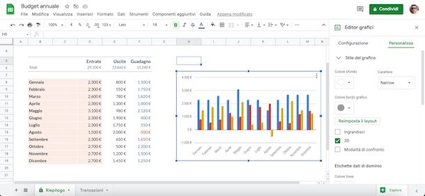
Complete the configuration of your chart, you can move on to customization. Then select the tab Customize and press on the options of your interest (Graphic style, Chart titles and axes, Serie, Legend, Horizontal axis, Vertical axis etc.) to change the style of the chart, add any titles, change the colors of the individual series, manage the legend and much more.

For example, if you want to change the colors of the chart, select the option Graphic style and set the colors of your interest through the options Background color, Graphic border color, Line color e Data label text color. In this section you can also edit the character used for chart labels and apply additional customizations, such as the ability to enable the 3D mode which allows you to view the graph data in 3D.

Once the customization of your graph is also finished, by clicking on it and pressing the icon of three dots, you can select the option Download to download it to your computer in PNG, PDF The SVG.

By choosing the options instead Publish chart e Publish you can publish the chart online as image or how interactive chart (in the latter case, updating the data in the Google sheet will automatically update the interactive chart as well). In both cases, a link will be generated to access the chart and you can also copy the HTML code to embed it on a website.

Finally, if you want to permanently delete a graph, click on the one you want to delete, press the icon of three dots and select the option Delete chart from the menu that is proposed to you.

How to make a chart on Google Sheets from the app

As you well know, Google Sheets is also available as a device app Android e iPhone/iPad. The operation of the app in question, including the creation and customization of charts, is almost identical to the version of Google Sheets accessible from a computer (although with many limitations compared to the latter).

Read This Now: How to turn off automatic brightness on Android - Easy Steps

After downloading Google Sheets from your device store, start the app in question and log in with your Google account. Once this is done, click on the button + located at the bottom right and select the option New worksheet, if you want to create a new blank spreadsheet, or Choose a model, if you want to create a spreadsheet from one of the ready-to-use templates. If, on the other hand, you have already created a spreadsheet, locate it in the section Last open for me and tap his Name, to open it in the app.

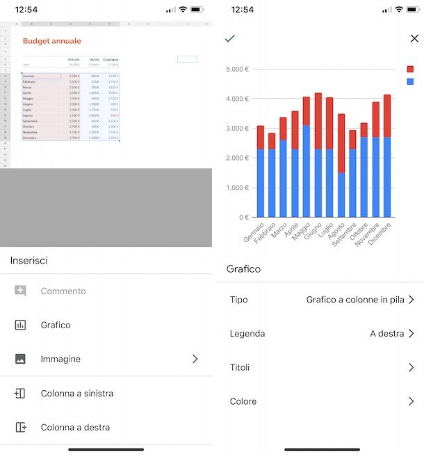
At this point, to create a new chart, select the cells containing the data of your interest, press the button + located at the top right and select the option Graphic from the menu that opens. In the new screen that appears, tap on the item Kind, to choose the type of chart you prefer (Line, Area, Column, bar, Cake, Dispersion etc.) and tap on the option Legend to indicate in which position to display the legend.

Then press on the item Title to add the titles of the chart, the horizontal axis and the vertical axis; select the option Color to choose the colors of the chart and tap the button ✓ to add the latter to the spreadsheet.

Now, press on the graph in question and drag it to the position you prefer, while keeping your finger pressed on one of the four corners and by swiping in or out, you can adjust its size.

If you want to change the look of the graph, tap on it and press the icon of pencil, top right. You must know, however, that it is not possible to change the data selected during the creation of the graph: in this case, it is necessary to delete the latter (you can do this by pressing on the graph of your interest and selecting the option Remove that appears on the screen) and create a new one.