How to Calculate the Percentage of Pass and Fail Correctly in Excel?

If you are a teacher in any of education levels It will surely be very useful for you to carry out statistical studies that allow you to know the development of your students; Among the most common data you have, for example, the calculation of the average number of students in Excel or the section, and for this you can use this program.

Although it is not the only thing you can use, since this tool will allow you to do many other calculations to evaluate the performance of your students. In this post we will show you how to calculate in Excel the percentage of successfully passed and failed.

How to use the functions that allow you to know the number of pass and fail?

If you are from the old school you will already know how to obtain the calculation as student grade point average and the section, as well as other variables manually; however, by using Excel, all calculations are simplified, making the process easier.

Allowing you to keep tables for electronic records of your students’ grades. In addition, you will have other functions to know the number of approved and failed students, such as:

SI function in simple format

The “IF” function is very useful for many applications, to make use of this function you need to know the structure or syntax it handles to place the correct argument. In principle, the function “IF” is a logical expression that is used to verify the veracity or falsity of a situation. For example, to evaluate whether a student passed or failed a certain course, you can make use of this function.

Suppose that the minimum passing grade for a student in a “Mathematics” course is 60 out of 100, then we can make use of this function to assess whether the student’s grade is in pass or fail.

The “IF” function requires the following arguments, “Logic_Test” This is the cell to be evaluated together with the evaluation criterion, “Valor_Is_Verdadero” in this space you can place text to indicate the situation in true condition.

On the other hand there is “Valor_SI_Falso” which is where the text or function corresponding to the result evaluated as false in the function will be placed. Assuming that you have a student who scored 62 out of 100 points, then the student must have a “Pass” condition, for this you must place in the evaluation cell “= IF (C3> = 60;” Approved “;” Failed “)”.

With the previous expression you are telling Excel that evaluate the grade located in cell “C3” and if this is greater than or equal to “60”, then put the label “Approved”, if the qualification is less than 60, then the label will be “Failed”. The result of the evaluation for the student “Pedro Pérez” will be “Approved”.

Consider that the “YES” function in simple format, can evaluate only the condition of a student, if you need to know the total number of approved and failed students, you will have to use the function “Count.If” that we explain below.

COUNT YES formula (rank: criterion)

This function will allow you to count a number of elements that meet a certain condition, the structure of this function “Count. If” will ask you to enter the “evaluation range” which is all the cells where you want to evaluate the possible existence of a condition. In addition, you must enter the criterion, which is the condition that you will be evaluating.

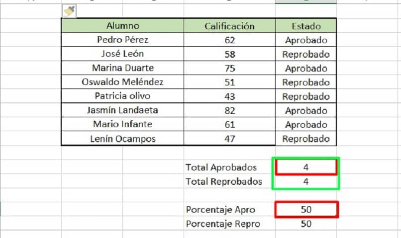
For example, if you have the table with the results of the students’ grades and their respective individual statuses, it is necessary to evaluate the total number of approved students, for this place in the evaluation cell the following “= Count.If (D3: D10;” Approved “)”, you are telling Excel to evaluate the range of cells D3 through D10 and count the number of “Pass” labels that exist.

To evaluate the total number of failed, put the same expression, but change the label “Approved” to “Failed”, with this you will be getting evaluate both labels or conditions that students may have.

How to calculate the percentage of students passed and failed?

Once you have obtained the total number of approved and failed students in the course you are teaching, you can obtain the percentage of students who passed the subject and the percentage of them who will have to repeat the course. For this you must know the total number of students in the course and then apply the rule of three to obtain these percentages.

In this first case, if you have 8 students in total, you know that those 8 students represent 100%, then the number of approved students corresponds to the percentage of approved students. The criterion of the rule of three is applied and you get the “Pass percentage = (No. Pass * 100%) / 8”Assuming there are 4 approved students, you will have a 50% pass rate.

If the list of students is very large, you can use the “Count” function and choose the range of cells where the names of the students appear, the formula will return the total number of students. Then you can apply the rule of three knowing the rest of the elements (Failed, approved) and you will have your percentages.

How to apply a conditional format to easily identify your students’ data?

Another way to evaluate the results or data of the students is to use the conditional format that the Excel tool offers, there are many modes of operation for the conditional format.

However, this time we will be addressing how change color in cells according to grades of the students. To do this you must navigate in the upper menu and follow the following steps:

• Search for “Start,” then proceed to choose “Conditional Formatting.”
• Choose the cells you want to apply conditional formatting to, and click on “Manage Rules” that is displayed when clicking on “Conditional Formatting”.
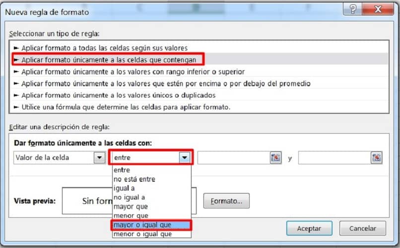
• Click on the “New Rule” button and in the pop-up window select “Apply format only to cells that contain”.
• Choose the second field that contains the list and navigate the list until “Greater than or equal”, then put the value in the third field, in this case it is “60”.
• Click on the “Format” button and navigate to fill in the top menu.
• Choose the color you consider appropriate for ratings greater than or equal to “60”, in this case we choose dark green.
• Click OK, then click OK again and you will have the first rule created.
• Now repeat the process and create a new rule, but instead of choosing “Greater than or equal to”, choose “Less than” from the list in the second field, likewise place 60 in the third field, and repeat the formatting process for the color. We chose red for ratings less than “60”.
• Finally, click on the apply button and you will see the changes that the cells undergo based on the established criteria.

As you may have noticed the process to establish labels that allow you identify pass or fail students In a certain course that you are teaching, it is easy to execute in Excel, in addition, you can learn how to make graphs in Excel in a simple way to show the results that were obtained at the end of your course.