How to Create a Pareto Chart Using Excel and Leave It Spectacular?

If you are the owner of a company and you are interested in addressing the problems associated with the productivity of your business, you should carry out an analysis of the causes that produce these problemsFor this you will have a tool such as the Pareto diagram.

Now, you can also count on another tool such as Microsoft Excel to make the graph you need, that is why we teach you how to create a Pareto chart using Excel. Continue reading and learn how to do it.

What should I use to create a pareto chart in Excel?

There are various tools in Excel that you can take advantage of to format your tables and get the best out of them, in the specific case of a Pareto chart, you will need to arrange the data in order to show the recipient in the best possible way and thus facilitate their interpretation. For this you can have:

Benefits of using ‘Class Width’

When you make a table where you present data for carry out studies of statistical elements such as frequency, accumulated frequency, mode, median, among others, it is usual that on certain occasions you group the data by ranges, this is known as class width.

That is, you will be able to make use of a range of input data, where you will add the elements belonging to that range of values ​​and later you will point to the frequency.

In the case of the Pareto chart in Excel you can opt for this technique, grouping the smallest problems in a certain item and adding the values ​​that correspond to it to obtain a more synthesized analysis. This will save time and make a shorter presentation of the data in the tables.

Advantages you will have when using ‘By Category’

Excel has grouping tools by category in its versions from 2016 onwards, so if you have one of these versions on your PC, you will be able to use this resource that will save you time and help you to classify the problems to make a simpler grouping.

Once you have the table with their respective problem descriptions, you can employ category grouping using the markers you require.

In general, you will see that you can use general values, percentage, accounting, currency, number, fraction, scientific and many more. This will allow you to give the format you need for your graphics to better represent the data.

You may be interested in using ‘Overflow class’

The overflow class is another of the tools offered by Microsoft Excel in its most recent versions, it is a method that allows grouping higher values in the same category or range. To access this tool you must right-click on your graph and navigate to the “Axis Format” menu, then check the “Overflow Range” box and place the number in the indicated field.

Underflow class may be what you are looking for

Similar to the overflow tool, it allows you to choose a range of numbers that are below a specified value and group them in the same category or item. Access this function by following the steps indicated in the previous section, but instead of navigating and checking the “Overflow Range” box, you must check “Sub overflow Range” and place the value in the indicated field.

This tool will save you time of analysis in your graphs and presentation of results. If you have any questions, visit Microsoft Excel technical support for more information on this.

You can also do it automatically

Another possibility you have is to use automatic formats in the construction of Pareto diagrams. By using this method you are telling Excel to use a single column of data to build the chartFurthermore, the class width will be determined by the program applying Scott’s reference rule.

This is how you should build a pareto diagram from scratch

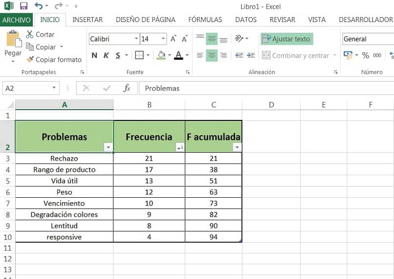
First of all you must make your data table and use it correctly, typically they are those where problems that you must address are represented. Organize the data by placing from highest to lowest those with the highest frequency of incidents, proceed to calculate the accumulated frequency and if you wish the accumulated percentage. Follow the steps below to get your diagram:

• Once you have your board prepared according to the indications given, choose the range of data you want to use to construct your Pareto chart.
• Navigate to the top menu and choose the “Insert” option, from here you will have two options. The first is to click on “Recommended Charts” in the left menu you should see a Pareto chart. If not, click on “All graphics” and choose “Combo box” Take the second option and you will have your Pareto chart.
• Proceed to give the formats you require to properly present the information.
• The second way you have to obtain your Pareto chart will depend on the version of Excel you have. In the most updated versions, you must navigate to “Insert”, then choose “Insert Statistical graphics” and then click on “Histogram”, you will be presented with several options among which you have “Pareto”, you choose that option and you will have your diagram.

Once you have your diagram you should evaluate the axes and the presentation of the informationIf you consider that it is okay, you will have finished your work, if not, you should consult the previous sections where we explain the resources to format your graph.

How should a pareto diagram look in Excel if you did it right? ( Example )

A well-prepared Pareto chart in Excel should have a main representation in columns placed in descending order, in addition, you will see a continuous line that joins the central points of each column, whose value corresponds to the accumulated frequency or accumulated percentage according to the needs you have.

Another important aspect in a diagram of this nature are the axes that represent the main value of the items represented by the columns and that are usually shown on the left side of the graph. Also, you will have the right axis of the graph where you will see either the cumulative percentages or cumulative frequency.

Is Excel the best tool for building pareto diagrams?

As a good calculation tool, Excel is a good option for make Pareto diagrams, however, it is important to mention that there are other tools that you can use to develop diagrams of this nature in a professional way.

Although to achieve this purpose you must have programming skills in various languages ​​such as Python, C ++, Visual Basic, among others. You can also use the following options:

Alternatives to Excel

As alternatives to this powerful tool you have the software where you should use programming like those mentioned above, as well as other environments such as iWork with its Numbers software that is used in macOS, or Google Docs if you want to work online.

In general, the most used tool and known for its power to develop many graphic resources, calculation and records is Excel.

The process to get your Pareto diagram is not complex, We hope that this post has been of great help to you, to complement it we can learn how to insert images with hyperlinks in Excel and we will surely consolidate the knowledge about this excellent program.