How to Put or Remove Leading Zeros with Excel? – Set Digits

Working with the Microsoft Excel tool can be very productive, since it will save us a lot of time when making calculations. But some basic functions like putting or removing leading zeros when we import data. If you do not have the slightest idea how to do it, then we will tell you how to put and remove leading zeros with excel.

What should you check before modifying leading zeros in Excel?

It is very annoying when zeros appear to the left of our figures and we need to be attentive to this detail. Since for different reasons, this problem can occur that completely changes the data that we want to enter in the table. Therefore, Before modifying the leading zerosyou should check if:

If you pasted them from somewhere other than Excel

It is possible that at the time of importing the numerical data, at the time of pasting it the do it somewhere other than excel. As a result, it will place zeros on the left side of the number, this is very common to happen. And for this reason you should always be aware of the place where you paste them.

When there are characters other than digits in the cell

Another aspect that you should check before modifying the leading zeros is when the cell where you placed the figures has another format. Therefore, when pasting, it recognizes data as characters other than digits. But do not think that this will be solved, if you change the format of said cell and what must be done is to transform the data.

What is the correct way to remove or add leading zeros in Excel?

Now, if in your spreadsheet show zeros to the left of the numbers, or, on the contrary, you want to add them. You can apply some methods from the basic functions and formulas that Excel offers us and in which we will eliminate the leading zeros or add them. For this we will use an example in which we will have column B with 6 numerical data ranging from B2 to B8.

Using the text function

We will show you first how to add zeros and for that we will use the text function, in this way we will change the format. Then we will position ourselves in cell C2, select it and write the formula =TEXT(B2’00000′). Then you press the Enter key and immediately the zeros will be displayed to the left of your data, repeat this step with the different cells.

Using ‘paste special’

Continuing with the example above, we will remove the leading zeros from the data, but now using paste special. To do this we just have to take the next column, that is column C and fill it with numbers ‘1’. This means that we will put 1 from C2 to C8, then copy all the values ​​from column B.

The next step is to position ourselves with the cursor on the first cell of column C, right click and in the menu we will choose the option ‘Special paste’. This action will show its window on the screen and in which we must select the ‘Multiply’ option. Then we click on the option ‘OK’ And that’s it, now we will see the data in column C, without the leading zeros.

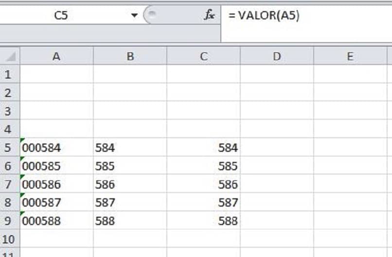
With the value formula

If you want to apply a slightly simpler and faster method, we will take the same previous example to be able to explain it clearly. In this case we are going to do use of ‘Value’ function which removes leading zeros that are taken as text. To use it, we must select the first cell of column C and write the formula =VALUE (B2).

this formula will remove leading zeros of the number that is located in column B2 and now shown in column C2. You must repeat this same step with all the rows of column B that have figures with zeros to the left. To do this you can use the keyboard to copy and paste the format.

Using cell formatting

We have already seen the different ways that we will have in our spreadsheet, to eliminate zeros that are placed to the left of the data. But you may want to add zeros and the best way to do it is changing cell format. To do this, we will select the cells that contain the numerical data and then right click.

In the menu that will be displayed, we must choose the option ‘Format cell’ and this action will generate a box on the screen. Next we select the ‘Custom’ option and then we go to the ‘Type’ option where a text box is displayed. In which we are going to write the number of zeros that will appear to the left of your numerical figure.

It should be noted that if you put 5 zeros and your data contains 3 numbers, only two zeros will appear on the left. If you want more zeros to appear you must go up the number of zeros in the ‘Type’ option.

Why does alignment continue to the left after removing zeros in Excel?

After the zeros to the left of the figures or data that you have placed in your column have been removed. These will continue to align to the left, because the Microsoft Excel program is taking as text and not as numeric values. But this can be fixed, if we just change the cell format and this can be to ‘Number’ or ‘General’.

Thus, we have presented you with different options that will allow you to remove or add leading zeros in a numeric data column. And as you have seen in a very simple and fast way, very similar to freezing the columns and rows in an Excel table. And we hope we have helped you and you can send us any questions through the comments box.