How to create a Microsoft Excel sheet that updates automatically

Are you continually changing the input data range of your Excel spreadsheet as new data becomes available? If so, the Excel charts that update automatically are a huge time saver. Charts help you make fact-based decisions in Excel. They are a nice change from looking at data and columns. They also aid in the decision-making process by allowing you to see your results where improvements may be necessary. The difficulty in handling data and graphs is that you constantly have to go back to the graph and update it to get new data. Creating charts in Microsoft Excel can seem overwhelming, but it’s easy to do and you can even create one that updates automatically.

In this article, we will guide you on how to make a chart in Excel spreadsheets that will automatically update when you need to add new data.

Steps involved in creating self-updating charts

We will use an example to show how to create a self-updating Excel spreadsheet. For this, I am creating a spreadsheet that will track the number of copies sold at a bookstore.

Step 1: create an Excel spreadsheet

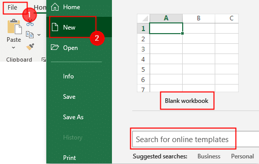
1. Open Excel. Click on File> New> Template or blank book.

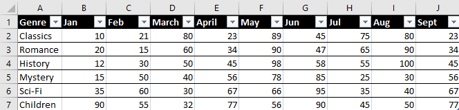
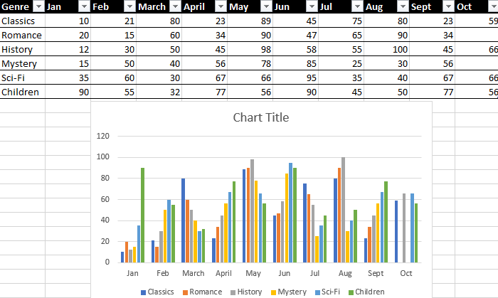
2. Now, start entering your data and create the spreadsheet. The final spreadsheet will be seen below.

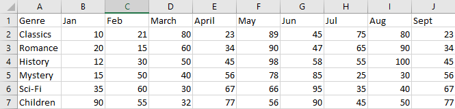
NOTE: Make sure each column has a heading once you enter your data. Your table and chart headings are crucial for labeling data.

Step 2: create a table.

Now, you need to format your source data in a table. To do that,

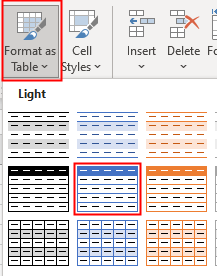
1. Select a cell in the data, Go to Format as tableand click the format you want.

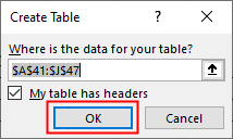
2. A pop-up window appears, leave everything as is and click it’s okay.

3. Now the source data is converted to a table shown below.

Step 3: insert the graphic

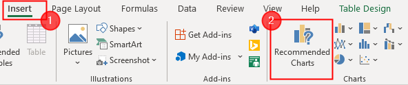
1. Select the entire table, go to Insert> Recommended graphics.

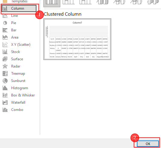
2. Select the type you want and click OK.

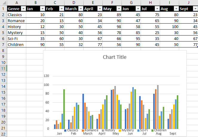
3. Now, the chart is created and displayed next to your table.

Step 4: enter the new data

By adding new data to the table, we can now see how well our chart works. Fortunately, this is the easiest step in the procedure.

Just add another column to the right of your existing chart to add new data. Because the format of the previous columns is preserved in the Excel table, your date will automatically match what you have entered so far.

The x-axis of your chart should have already adjusted to fit the new input. Now you can enter all your new data and the chart will instantly update with the new data.

The ability to create time-saving, self-updating sheets is one of the most powerful features of Microsoft Excel. This can be as simple as making a basic auto-update chart, as demonstrated here.

That is all.

I hope this article is informative. Comment below on your experience.

Thank you for reading.