How to Make Graphs in Excel from a Table with Various Data? – Steps to follow

The Microsoft Excel tool is one of the main ones to perform calculations as a company’s budget. However, their application is not just limited to running calculations, but you will also be able to obtain graphs that will make your work of data interpretation easier.

So in this post we will show you how to make charts in Excel from a table with various data. Go ahead and learn how to do it.

What types of charts can be made in Excel?

Excel offers you different types of graphs so that you can use the one that you like the most or suits the nature of the topic that you are analyzing. Before starting the process to obtain the graph, you must have the data organized in the table.

Pie chart

It is one of the most common graphs that you will find in Excel, its shape as its name indicates is a cake where the portions represent a piece of information with the quantity and corresponding percentage. To obtain this graph follow the steps below:

• Choose the data ranges from the table that you want to graph.
• Navigate to the tools tab and click on “Insert”.
• Choose the type of graph “Circular or donut”, take the first of the “Circular 2D” options.

As you may have noticed, the pie or pie graph will be displayed with the portions of the pie representing the amount that corresponds according to the data you have selected. Here you should keep in mind that if you put the header data they will appear in your graph.

Bar graph

This type of graphics displays sketched data from tables as bars Identified with series names and corresponding quantities, typically you will see each horizontal bar in different colors for each item in your table. The steps to obtain this type of graph are basically the same as the previous graph

• Select the data from the table that you want to graph.
• Navigate in the toolbar and choose “Insert.”
• Search as the type of graph to choose the “Bar Graph”, and take the model that you like the most.

Comparative graph

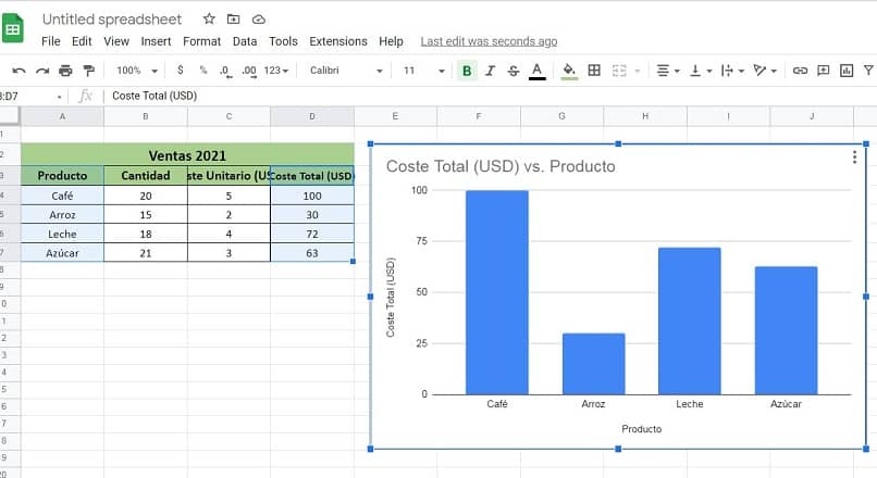
This type of graph is very useful for making comparisons between variable values ​​that have changed Over time, for example, a classic application is the sales of a company in consecutive years. In comparative graphs, we recommend using column-type graphs, since it allows you to better present the comparison between the data you handle.

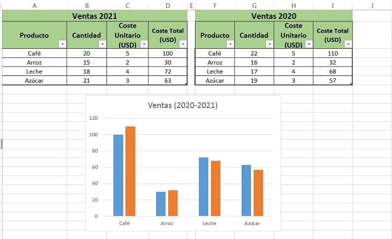
Remember that you must navigate in the toolbar and choose “Insert”, then you go to the type of chart and select “Column chart”. At this point you have two options to finish your work.

The first is to choose the “Products” data and press “Ctrl”, keep it pressed and with the mouse select “Total Cost” for example, or “Quantity”, it depends on the value you want to graph.

You will see that when selecting the column chart it will be displayed only with the values ​​for a table, then you must right click on the chart and choose “Select data”, a pop-up window will appear where we select “Add”.

In the field corresponding to the series name you must choose the range of “products” and in the field of series values ​​choose the range of “Total Cost”, both table ranges that have not been worked. Click on accept and you will have your graphic ready.

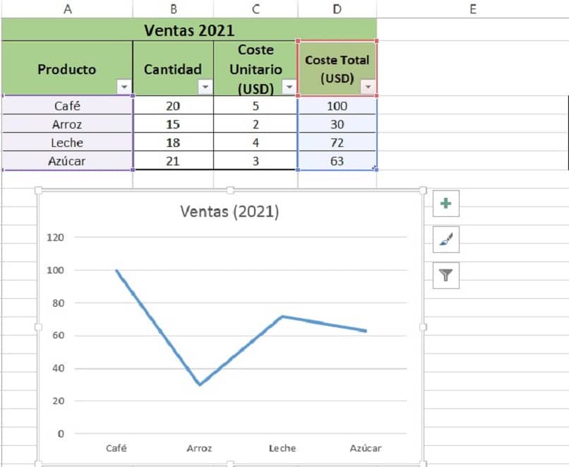
Line graph

This type of graph is formed with continuous or segmented lines that show the evolution of one or more variables over time. You can give it many applications in various fields of study, from lines of moving average in scientific studies, to other representations in fields of economics, finance and others.

The procedure to insert this graph is the same as above, you only have to select “Line Graph” when choosing its nature.

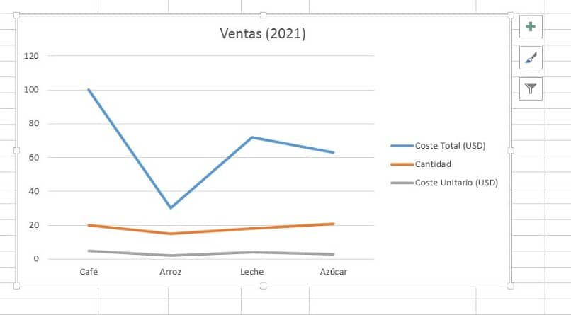
Graph with variables

The comparison chart is a type of chart with variables, and why? Simple you are driving more than one variable on the same graph, so you can see that these are resources that allow you to analyze two or more variables at the same time. To implement this kind of resource you must follow the steps mentioned in the comparison chart.

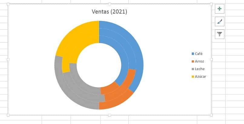
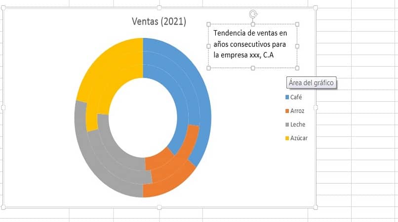
Donut Chart

The representation of this resource is done through rings instead of portions like a cake, this type of resource allows obtain segments of the ring that represent the change of a variable in time, in addition, like other graphs with this you can represent several variables in the same space, resulting in several circumscribed rings. Follow the same steps for the chart types above and choose “Donut Chart” to get your resource.

How to create a chart in Excel with one or more variables from a PC?

Generally it is more comfortable to work with programs like Microsoft Excel in computers, laptops or equipment of a similar nature. However, depending on the OS (Operating System) that you have installed on your computer, the process will be a little different. There are even those who prefer to collaborate online for which it will be very useful to work with Google Office, specifically Google Sheets or Excel spreadsheet online.

If you do not know this tool, you can see the characteristics, similarities and differences of Google Office with respect to Microsoft Office, so you will determine if it will be useful at any time for your activities. Now, taking into account consider the type of OS or if you will work online, Let’s see the differences that you must take into account to obtain your graph in Excel.

In Windows

It is one of the most used OS worldwide, that is why it is very useful to know how to make your graph in Excel, to do this, follow the following steps:

• Open the Microsoft Excel application.
• Create your table with the data you want to process and obtain your graph.
• Select the data you want to plot.
• Navigate to the toolbar and click on the “Insert” button.
• Choose the type of graph you want to obtain (Linear, bars, pie, columns, rings, among others).

On macOS

MacOS is another of the most used OS worldwide. Basically the steps to obtain a graph in this operating system are the same steps that are carried out to obtain your graph in Windows. That is to say, the key is in the handling of the previous table with the data that you have to handle, taking into account that said data must be well organized. The rest of process is the same as the previous section.

From the web

To get your chart in Excel or Google Sheets from the Web, you need to enter the document, whether it has been shared with you, or whether you are the owner of it. In any case, it is a document that you must drive from Google drive, and once you have defined the data from the table that is the starting point, you can perform the following steps:

• Select the data previously organized in the table that you want to graph.
• Navigate in the top menu and click on “Insert”.
• Choose from the drop-down menu the option “Graph” or “Chart” depending on the language configuration of your drive.

By doing the previous steps you will get your graph, however, by default you will get a column graph. If you want to change the type of chart, you must navigate to the “Chart editor” or “Chart Editor” menu and click on the “Setup” option. You will see that you will have the option “Chart Type” or “Chart Type” where you can choose the type you want.

How to make a chart with Excel from a mobile device?

Making graphs in Excel from mobile devices is possible, although the process is more complex than doing it on PC. For this of course you must have the corresponding app according to the OS of the mobile you have available. Here we show you how to do it in the most popular ones.

Android

It is undoubtedly one of the mobile OSs most used by users, in this case for get your Excel chart, in principle you must have the app installed. If you don’t have it, proceed to download the Excel app: view, edit and create spreadsheets from the Play Store.

• Open the Excel application on your Android.
• Choose the file where you want to plot the data.
• Select the data ranges in the table that you want to process.
• Navigate in lto the toolbar and click on “Insert”.
• You will see a submenu where you must choose “Graphic”.
• Click on the type of graph you want to display and that’s it.

iOS

• Open the workbook where you want to run the chart.
• Select using the corresponding controller button the ranges of data to be plotted.
• Click on the edit button and navigate to the toolbar tools to click on “Insert”.
• Find the option “Chart”, then click on “Type of chart” and that’s it.

Windows Mobile

• Identify and open the file that you are going to work on to obtain your graph.
• Choose the data ranges to plot using the corresponding select controller button.
• On your Smartphone, press the plus button (…) and then select “Home” to navigate to “Insert.”
• Select the “Chart” button from the submenu that appears.
• Choose the type of graph you want to show in your spreadsheet and you’re done.

How do you add a text box to a chart?

Sometimes it is important display supplemental information as text on charts in order to facilitate the interpretation to the reader. That is why we show you below the process to insert text boxes in Excel charts.

• Once you have obtained the graphic you are working on, select the option “Insert” in the upper navigation menu.
• Click on “Text box”.
• Select the area of ​​the graphic where you want the text message you are placing to appear.
• Write your message and once you finish, press the “Enter” key on the keyboard or press outside the text box.

In conclusion graphics are very powerful and useful resources that can be used in Excel spreadsheets in any of its versions and for any device or OS. We hope this information has been helpful to you and we invite you to continue visiting our tutorials and post.