How to Toggle Color Between Rows and Columns in Excel to Make It Look Better?

In this article we invite you to put aside the tedious practice of marking the cells you want to highlight one by one; instead you will automate the shading of Excel columns or rows depending on their content, using tools such as conditional formatting, residual formula, among others.

How to shade an entire row or column without any macro?

To shade a strenuous number of columns or rows automatically without resorting to time-consuming methods that we probably don’t have. It’s necessary that:

On the one hand, if what you need is to shade a column, position yourself in the top cell of your column, simultaneously press (Ctrl + Shift + down arrow) and shade with fill color. On the other hand, if what you want is to shade an entire row, locate yourself in the first cell of your row, press simultaneously (Ctrl + Shift + right arrow) and color the cells in the row with ‘fill color’.

How to set skip rows of different color?

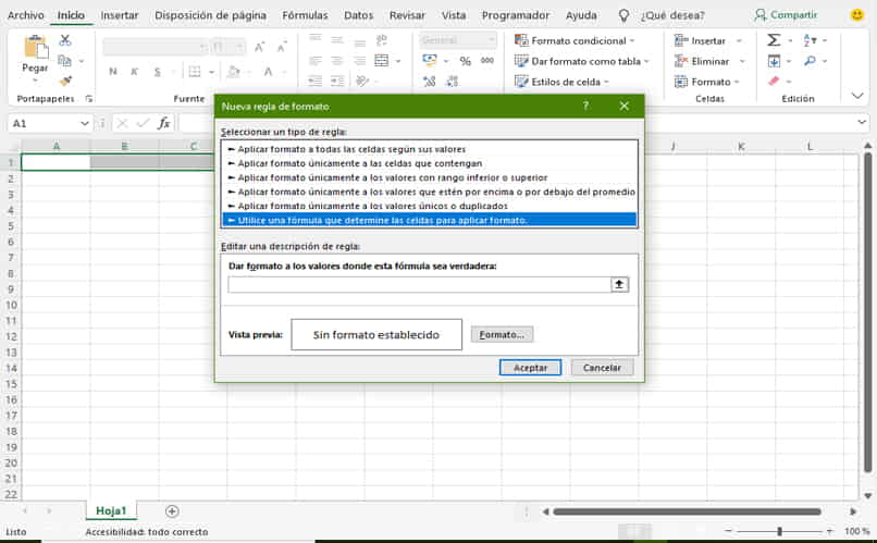
If what you want is organize your table with different colors according to its contentYou just have to: 1. Select the table without the header. 2. On the Home tab, choose the ‘conditional formatting’ option. 3. Click on ‘new rule’, determine the option ‘format the values ​​where this formula is true’, 4. Define the shading color in ‘format’ and write the condition that you want to color specifically in the description of the rule.

The condition can be determined to the numerical values ​​of a cell, for example if e2 = 3, it will be painted according to the color you selected in shading. The process can be repeated as many times as you want according to the content of your table in Excel and it will be shaded with the colors you choose.

Where can you change the format of the rows in Excel?

Similarly, you can change the format of the rows in Excel just by using tools, such as: the Residue formula or using a filter that will allow you to group your data according to its content.

Use the formula ‘WASTE’

The RESIDUAL function in Excel aims to know if a number is odd or even in a cell by dividing by 2; Therefore, it must be formulated as follows = RESIDUE (CELL; 2) = 0, making all the even numbers give 0 and the odd 1.

If what you want is to color the parts, go to the home tab, click on conditional formatting, new rule, in the pop-up window choose ‘use a formula that determines the cells to apply formatting ‘

In format define a color and write the formula in ‘format in cells where this formula is true’, for example: = A2 (Cell where the Residual is) = 0. In this way rows will automatically be marked pairs of your document.

Use a filter

If what you require is group the rows by a specific colorDo not despair, it is very easy to do it automatically with the filter tool, you just have to: 1. Go to the home tab of your Excel document. 2. Press the ‘sort and filter’ tool. 3. Choose ‘Filter’. 4. On the header there will be some icons with a downward arrow, press the icon and select the value from the drop-down list that you want to filter.

How can you use conditional formatting on an entire row or column?

Next we will teach you to use a conditional format that will allow you to highlight the entire row or column if a condition is met. For example: If you have an inventory control table in Excel of your company (product / unit / stock) and you want it to be marked as one color all row when sold out the existence of the products, you should only:

Go to the upper tab ‘home’ of the document, select the table you want condition without the headers, choose the option ‘conditional formatting’, click on ‘new rule’, choose to ‘use a formula that determines the cells to apply a format’, press the ‘format’ button to define the shading of the row.

Next, choose ‘format values ​​where this formula is true’ and pose the condition. For example: I want row A2 to be shaded when row D2 is equal to 0, for this I select with the cursor the cell (= $ D $ 2 = 0), edit the formula by removing the dollar sign which is between D and 2.

Otherwise, the formula would be fixed in cell D2, preventing the other cells from identifying whether the condition is met or not.